Enterprise import pipelines that rely solely on hand-user validation rules carry a structural blind spot. They only catch what their users anticipated. Statistically improbable but syntactically valid records, a junior developer’s salary entered at an executive rate, a pension contribution reversed in sign, a self-referential reporting line in an HR onboarding life, routinely pass every rule check undetected.
This article presents a hybrid validation architecture built on .NET 9 and ASP.NET Core, that pairs a lean custom rule engine with two unsupervised ML models: Convolutional Autoencoder and an Isolation Forest to generate a probabilistic anomaly score for every imported record. Both models run entirely in-process via ONNX Runtime inside a channel-backed background service pipeline, with no Python sidecar or external inference server required. Evaluated on 250,000 payroll and 180,000 HR onboarding datasets, the hybrid system achieves a ROC-AUC of 0.943 and an F1 score of 0.899, while cutting the hand-authored rule set by 61.7% and sustaining the throughput of 890,000 records per hour on a single commodity node.
Prerequisites
You need. NET 9 SDK, Python 3.11, and SQL Server 2022 (or PostgreSQL 16) installed on your system to work with the code example in this article. When you install Visual Studio 2022 (v17.10+), you can install the .NET 9 SDK at the same time through the Visual Studio installer. Alternatively, VS Code with the C# Dev Kit extension works equally well on my platform.
The core NuGet dependencies EPPlus, Microsoft.ML.ONNXRuntime, FluentValidation, , and OpenTelemetry will be installed from NuGet, while the Python training packages (scikit-learn, PyTorch, and skl2onnx) are installed via pip and are only required if you intend to retrain the models rather than use the pre-exported .ONNX files provided in the companion repository. The full source code for this article is available on GitHub
Validation Problem
Data quality is a problem from the start. Many companies know about it, and few fix this problem. There is a difference between having a system to check data and actually catching bad data. Most teams do not realise how big this gap is. The problem shows up later in salary payments, compliance issues and wrong financial reports.
The standard response is to write more rules. This works up to a point. After a few years of reactive additions following incidents, most enterprise import pipelines carry 40 to 60 validation predicates, many of which overlap, some of which conflict at edge cases, and all of which lag behind the business logic they were meant to encode. Nobody removes the rules that became redundant after a schema change. This accumulation rule applies to debt, which compounds exactly like technical debt.
Machine learning offers a variety of perspectives. A model trained on historically clean import data learns the multivariate distribution of valid records. It does not need an explicit predicate for every defect class. It flags records that deviate from learned normality, regardless of whether any developer anticipated that exact form of deviation. The practical challenge is integration, how do you embed ML inference reliably inside a transactional .NET enterprise pipeline without sacrificing throughput, auditability, or your existing validation infrastructure?
This article answers that question with a concrete architecture applied to real-world payroll and HR import workloads. All code snippets are drawn after testing on real datasets.
Rule-Based Validation
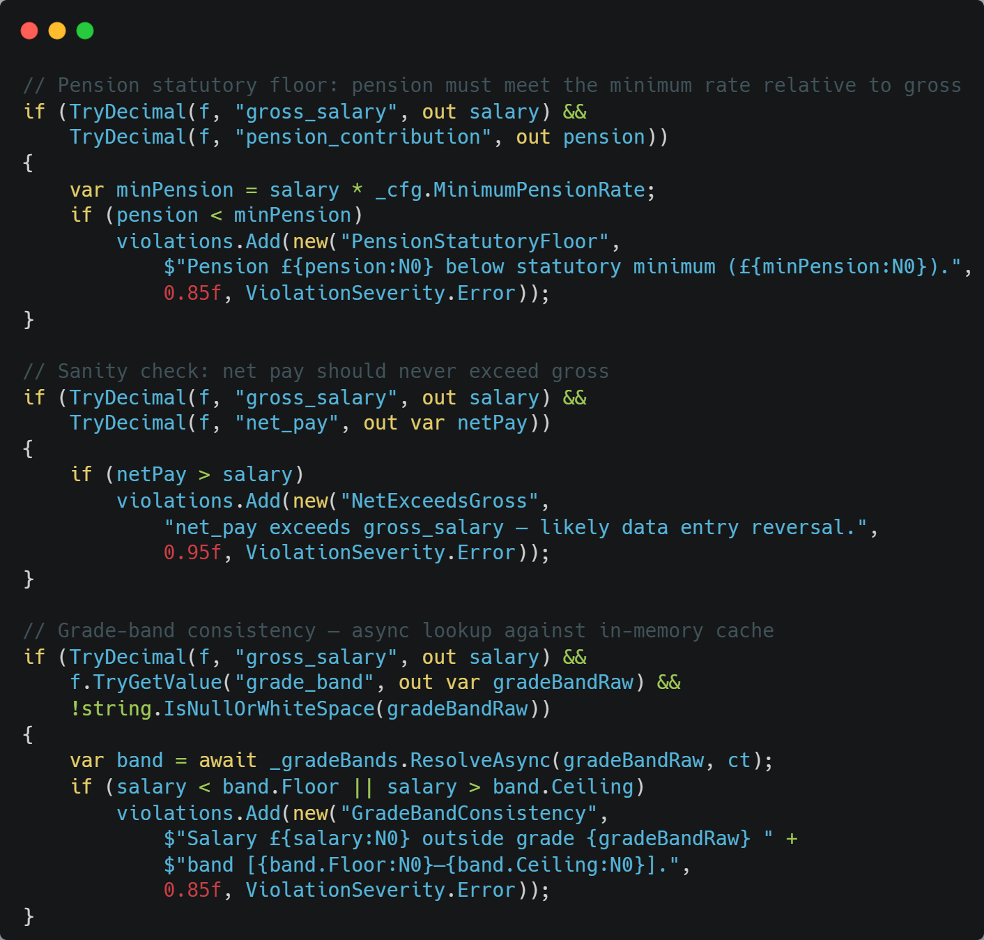
Take a real payroll import: employee_id, grade_band, gross_salary, pension_contribution , fte_ratio, net_pay. Rule set checks the things like:
- gross_salary >0 and within the company cap
- fte_ratio between 0.1 and 1.0
- pension_contribution above the statutory minimum relative to salary
- net_pay doesn’t exceed gross_salary
This type of rule handles the structure problem well. But they don’t catch a grad 3 employee earning a grade 7 salary, because that’s the relationship between two fields that changes every time HR restructures the grade bands. You could write a cross-field rule for it that we did, and it’s in the codebase repository. But then you’re maintaining a lookup table of grade-to-salary ranges that’s out of date within six months of any company.
The ML models cover this without a lookup table. They just know that grade 3 at $60,000 doesn’t look like anything in the training data, and they flag it. That’s the gap this architecture closes.
Architecture Overview: Three Signals, One Score
The core idea is straightforward: apply both models and run the rule engine against every record, then combine their output into a single composite anomaly score between 0 and 1.
- Rule Violation Score: denoted by S_rule which comes from the rule engine. These violations are weighted by severity, and multiple violations compound. A mandatory field failure carries a weight of 1.0 and dominates the score regardless of what else fires.
- Autoencoder reconstruction Score: denoted by S_AE, which comes from the autoencoder. The network learns to reconstruct clean records from a compressed latent representation. When it struggles to reconstruct a record accurately, that reconstruction error becomes the anomaly signal. This is best at cross-field covariation violations. Such cases where individual fields are valid, but their combination is something the model has never learned to encode cleanly.
- Isolation Forest Score: denoted by S_IF, which comes from the Isolation Forest, trained on two years of accepted clean import records. Records that sit in sparse regions of feature space, which unusually field combinations that the model rarely saw during training get high scores. This is particularly good at catching grade salary inconsistencies and near duplicate records with permuted identifiers.
The composite formula, as implemented in the AggregationWorker class, is:
SComposite=α*Srule+β*SIF+γ*SAE
Default weights are = 0.35, = 0.35, = 0.30, read from configuration via IOptions<ValidationWeights>. They’re tunable per import template. If you’re running a compliance-critical pension adjustment import, raise . If you have an abundant, clean history for a given template, raise and .
Below are the decision tiers:
| Score Range | Decision | Action |
| S<0.40 | Accept | Record committed to the import queue |
| 0.40≥S≤0.70 | Review | Held for human data steward review |
| S>0.70 | Reject | Excluded; structured rejection report generated |
The review tier is the most important design decision here, not the models. So, binary accept/reject forces you to pick a threshold that either misses anomalies or generates too many false rejections. The middle tier routes uncertainty to a human who has the context to make a decision.
Implementation in .NET 9
System components and technology stack: the production system is implemented entirely within the .NET Core 9 ecosystem.
| Component | Technology |
| Web API | ASP.NET Core 9 Minimal APIs |
| Excel Parsing | EPPlus 7 (streaming mode) |
| Rule Validation | FluentValidation 11 |
| ML Inference | Microsoft.ML.OnnxRuntime 1.17 |
| Background Processing | IHostedService / BackgroundService |
| Inter-service Messaging | System.Threading.Channels |
| Feature Engineering | Custom .NET pipeline; Accord.NET for stats |
| Result Persistence | Entity Framework Core 9 + NoSQL |
| Observability | OpenTelemetry + Prometheus + Grafana |
| Configuration | Microsoft.Extensions.Options (typed) |
Background Services Pipeline
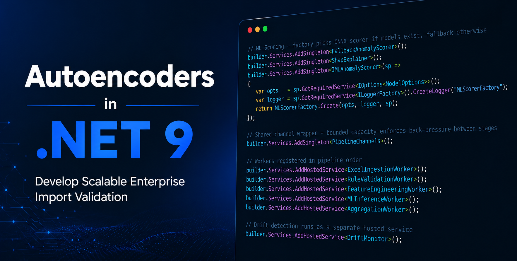
The system goes through the background services workers registered in order of Program.cs, each connected to the next through a bounded System.Threading.Channels.Channel<T> owned by a PipelineChannels singleton.
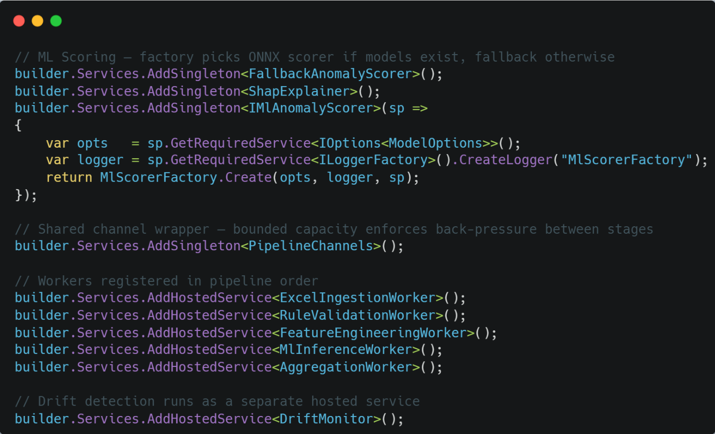
So, the PipelineChannels holds all the channels in one place and keeps the worker constructors clean. They just take the channel wrapper rather than the individual Channel<T> instances. MlScorerFactory It is worth calling out that it checks whether ONNX model files exist at startup. If they don’t exist, then the first deployment in cold environments
Rule Validation (Custom Weighted Validators)
We deliberately didn’t use Fluent Validation’s AbstractValidator<T> here. What we needed was direct access to per-violation severity weights so the pipeline could compute S_rule itself. So, each validator returns a typed List<Ruleviolation>, each carrying a rule name, message, weight, and severity.
The payroll validator’s tier 3 is on cross-field consistency, so this section mostly interacts directly with the ML layer.
The HR onboarding validator HrOnboardingValidator follows the same pattern and covers domain-specific cases like leaving entitlement below the statutory minimum, probation periods inconsistent with contract type, starting date predating the company’s founding, and one that sounds obvious but appears in real import. So, the employees listed themselves as their own line manager.
These rules are the ones we kept after both models were in place. All hard regulatory or structural constraints where you genuinely can’t substitute a probabilistic signal for a deterministic check.
ONNX Model Inside a Services Pipeline
The model uses MlInferenceWorker sits at stage 4 of the pipeline. It read FeatureRecord items from the channel, groups them into micro-batches (128 records, which is configurable in appsettings.json), and calls IMlAnomalyScorer for both model scores before writing ScoredRecord items downstream.
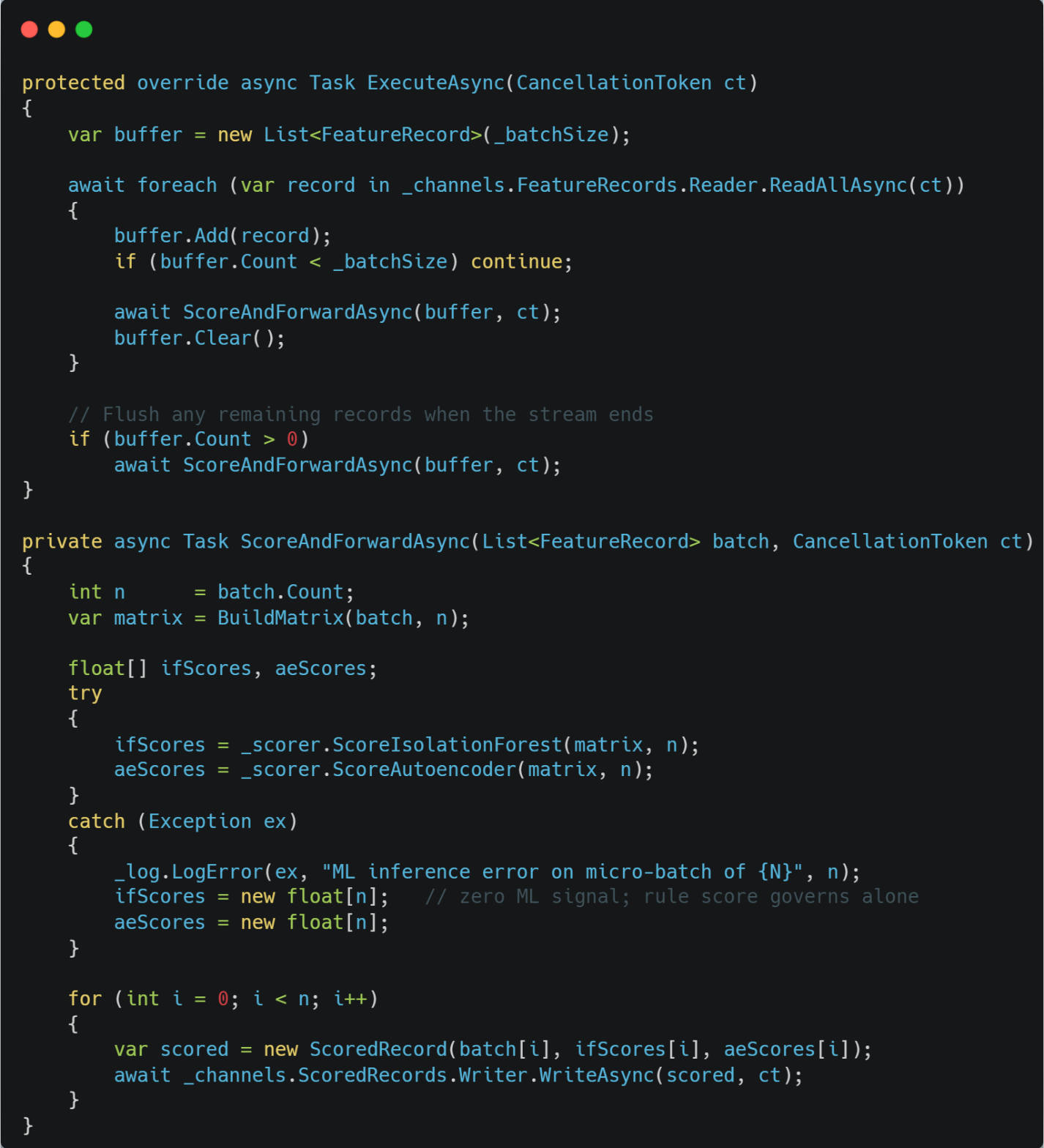
The try/catch matters more than it might look. ONNX sessions can fail when a model file is updated mid-deployment or when an input shape doesn’t match the model’s expectations. Rather than crashing the worker and stalling the whole pipeline, we set the ML scores and let the rule score carry the decision for that batch. It goes, it’s visible in monitoring, and operations can investigate without a service restart.
What the ONNX Scorer Actually Computes
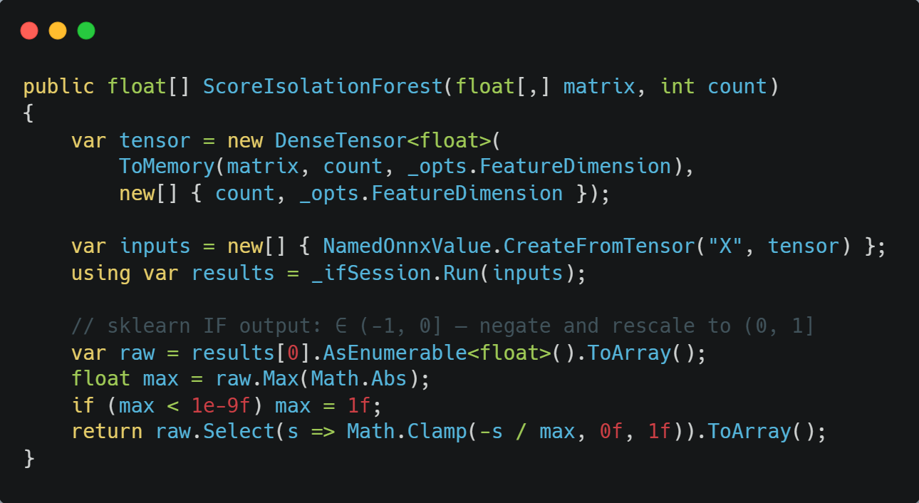
The class ONNXAnomalyScorer holds two pre-warmed InferenceSession objects and implements IMlAnomalyScorer. One subtlety worth knowing, sklearn’s Isolation Forest ONNX export produces scorers in the range (-1, 0), where more negative means more anomalous. The scorer negates and normalizes there to (0, 1) before they leave the method.
For the Autoencoder, the scorer computes the mean squared error between each input record and its reconstruction, z-scores that error against calibration statistics collected on a hold-out clean validation set, then runs it through a sigmoid. Clean records cluster around 0.5, genuinely anomalous ones push toward 1.
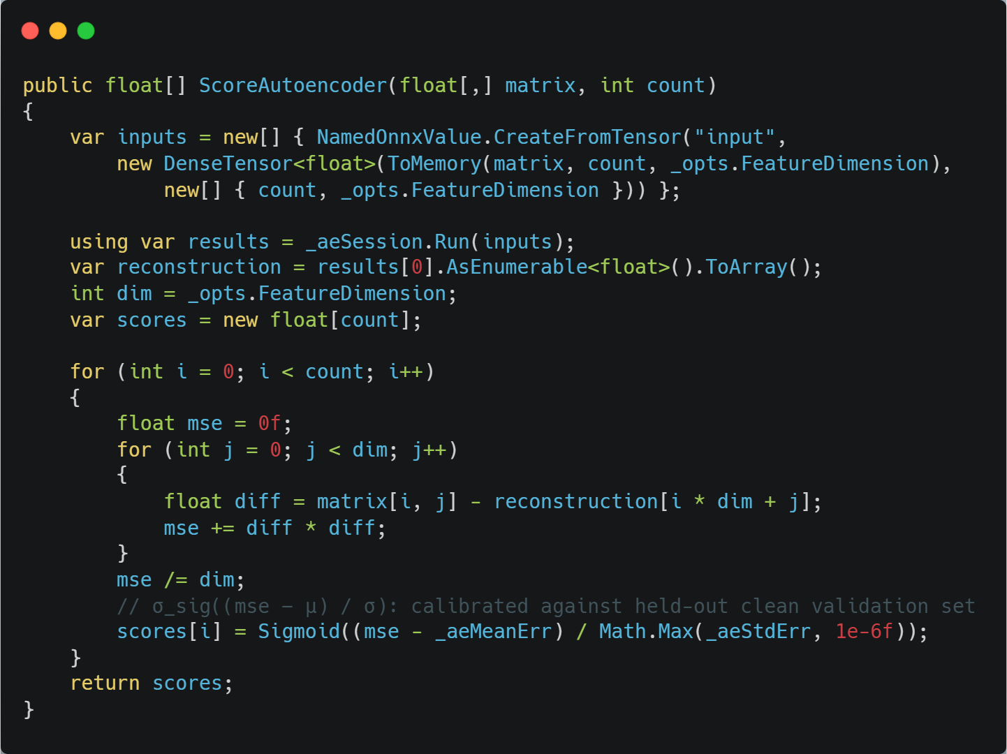
Calibration values (_aeMeanErr, _aeStedErr) come from appsettings.json Under the models section, set once after training using the validation set reconstruction error distribution.
Combining Scores and Persisting the Audit Trail
We apply the weighted formula on AggregationWorker, which routes each record into a decision tier, that is, computes the SHAP explanation that tells the data steward exactly which features drove the ML signal.
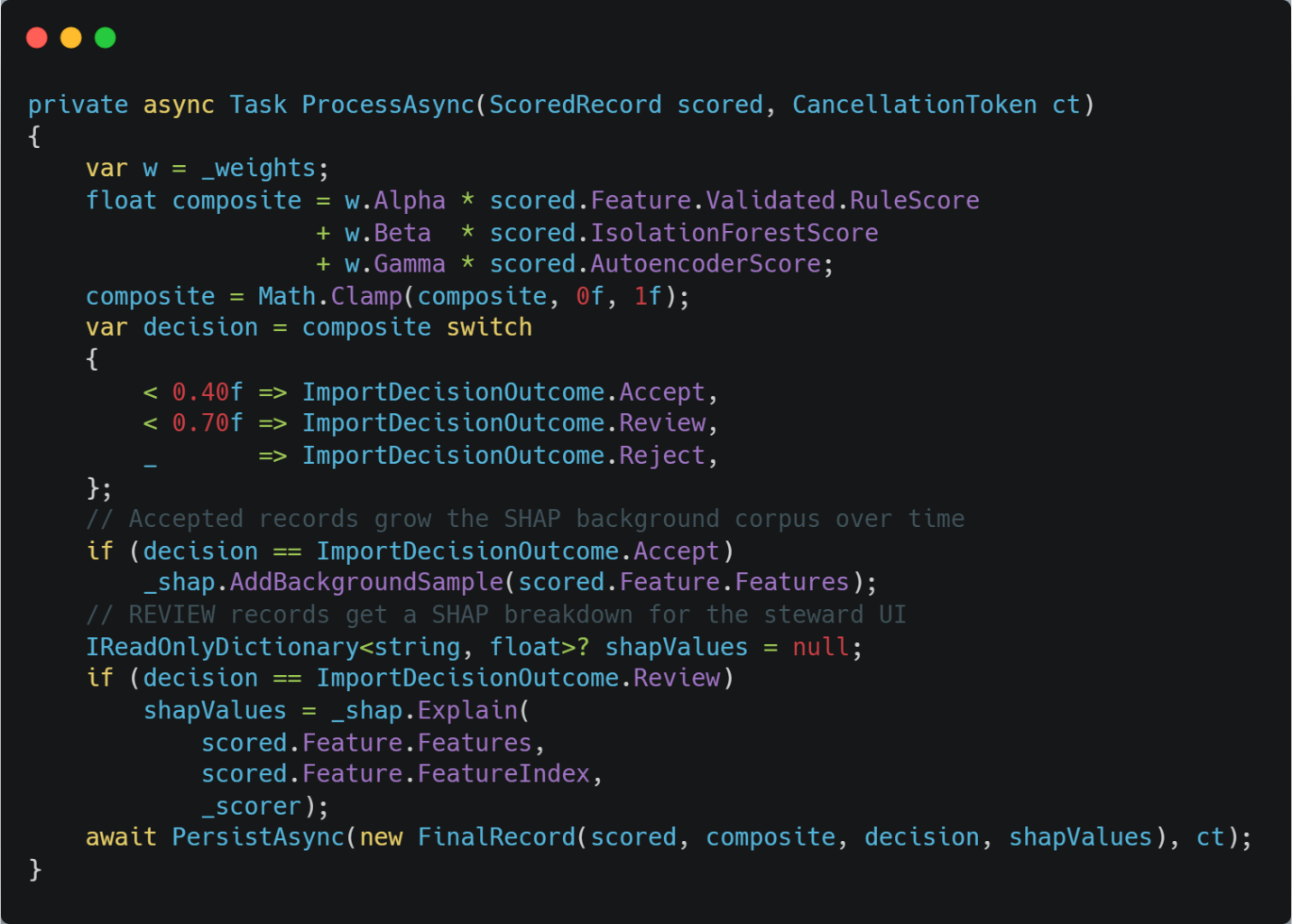
Each record gets a database audit entry via EF Core, containing the full score vector (RuleScore,IFScore,AEScore,CompositeScore, triggered violation rule names, and for the REVIEW tier records, the top SHAP feature contributions sorted by absolute value. When a data steward opens a flagged record, they see something like effective_hourly_rate :0.43,pension_rate:0.21, which is just not a number. That’s what makes the ML signal actionable rather than opaque.
Offline Models Training and Deploying via ONNX
Trained both models in Python with two years of accepted clean records, which have around 700,000 payroll rows and 550,000 HR onboarding rows. A few features of engineering decisions are worth highlighting because they affected model quality significantly.
The high-cardinality categorical fields like job_code where encoded using target encoding against anomaly prevalence on the training split. One encoding would have added over a thousand dimensions and made the Isolation Forest’s random partitioning almost meaningless. Continuous fields were scaled with RobustScaler rather than StandardScaler. So, the median normalisation is less sensitive to the genuine tail variation you see in senior compensation bands. Two cross-field features were engineered pension_rate and effective_hourly_rate, salaryFTE*1820. These capture exactly the cohort-level covariation that individual field rules struggle with.
The Isolation Forest used 200 trees with contamination, exported via sklearn-onnx. The Autoencoder convolutional encoder layers (filters:64,32;kernelsize=3), a 16-dimensional bottleneck, a symmetric decoder, trained with Adam and early stopping, that was exported from PyTorch via torch.onnx.export. both were validated numerically against their Python originals before going anywhere near production.
Results
Evaluation ran against two synthetic datasets, where we have 250,000 payroll records and 180,000 HR onboarding records with controlled anomaly injections across five defect classes, including grade-salary and inconsistencies, negative pension contributions, impossible FTE ratios, and copy-paste duplicates with permuted IDs, and statistical outliers more than five standard deviations from the grade-cohort mean.
| Configuration | Precision | Recall | F1 | ROC-AUC |
| Rule (47 rules) | 0.981 | 0.634 | 0.770 | 0.817 |
| Isolation Forest | 0.843 | 0.871 | 0.857 | 0.912 |
| Autoencoder | 0.819 | 0.894 | 0.855 | 0.908 |
| Hybrid | 0.912 | 0.887 | 0.899 | 0.943 |
The recall of 0.634 on the rule configuration means one in three anomalies gets through undetected. That’s not a theoretical concern, its real operational problem in payroll where a missed anomaly might not surface until the pay run. The hybrid brings that up to 0.887 while holding precision at 0.912, which is the balance you need when false positives have real operational cost.
The rule reduction result matters as much as the detection metrics. By raising the ML weights progressively and pruning rules that the models were already covering, we maintained F1≥0.89 with 18 rules instead of 47. That 61.7% reduction means fewer things to update when business policy changes, fewer edge-case conflicts, and a validation layer that’s possible to reason about.
On throughput 890,000 records per hour on a single node with no GPU, scaling near-linearly across additional nodes. A 250,000 payroll records batch finishes in under 18 minutes. ONNX inference p95 latency per 128 records in a micro batch came in at around 19ms.
Dealing with Model Drift Before It Becomes a Problem
One thing that bites teams who deploy anomaly detection models and forget about them, for instance, the business events shift the distribution of clean data silently. A salary uplift across 3,000 employees, a grade restructuring, and a new pension scheme. Any of these can cause models trained on last year’s data to start flagging legitimate records. There’s no error, no exception. Just a rising review rate that looks like a data quality issue, but is actually a model staleness issue.
The system includes a DriftMonitor, a hosted service that runs a test comparing the rolling 7-day distribution of ACCEPT-tier S_IF and S_AE scores against the training time reference distribution. When that test returns p<0.05, It triggers an automated returning pipeline. The Accept-tier Records from the preceding 90 days from the new proxy clean corpus, models are retained offline, and shadow deployment validates against a held-out recent window before promotion. In a simulated 18-month run, retraining triggered roughly every six weeks per model. That’s a manageable cadence.
Is this the Right Approach for your Team?
This architecture works well under specific conditions that are worth being honest about.
You need sufficient clean historical data. Both models need a meaningful corpus to learn from. Fewer than 50,000 verified, clean records, and the signal degrades. If your import history is sparse or you can’t confidently distinguish historical clean records from undetected anomalies, the ML layer won’t pull its weight.
You need distributional anomaly classes. If your imports mostly fail on missing required fields or type mismatches, a well-maintained rule engine handles those well, and the ML overhead isn’t justified. So your team needs to own the model lifecycle. Training, calibration, drift monitoring, and periodic retraining are ongoing responsibilities. Not large ones, but they don’t exist with a pure rule engine, and they shouldn’t be treated as a one-time setup.
You need a staffed review process. The REVIEW tier delivers value only if someone acts on flagged records. Without a data steward queue, you’ll need a more aggressive accept threshold, and you’ll lose some of the precision recall flexibility the three-tier model gives you.
What We Actually Learned Building This
The most valuable outcome wasn’t the improved detection accuracy. It was the 61.7% reduction in rules we no longer had to maintain. A validation layer with 18 well-reasoned, regulatory-grounded rules is something a team can own, understand, update, and extend confidently. A 47-rule validator with accumulated context debt is a liability.
The ML models do something rules never will, they get better as more clean data accumulates, and they adapt through retraining as the business changes. The rule engine stays static until someone updates it. Combining both means you get the auditability and regulatory certainty of explicit rules where you need them, and the adaptive coverage of statistical learning everywhere else.
If you’re running large-scale import pipelines on .NET 9 and you’re tired of writing the forty-eighth rule after the forty-seventh incident, this is a reasonable path. The ONNX runtime integration is solid, the Background Services pipeline model handles the concurrency cleanly, and the three-tier decision structure gives you a practical workflow that your team and your data stewards can operate.
Key Takeaways
- Rule engines and ML anomaly detection cover different failure modes. Rules are authoritative on structural and regulatory constraints. Isolation Forest and Autoencoder models catch distributional anomalies that no finite predicate set can enumerate. You need both, and they should run together.
- The REVIEW decision tier matters more than the models themselves. A three-tier system (ACCEPT, REVIEW,REJECT) routes genuinely uncertain records to human judgment instead of forcing a premature automated decision. This is what makes the ML signal practical in production rather than a liability.
- ONNX runtime makes in-process ML inference a native .NET 9 feature. Models trained in scikit-learn and PyTorch export cleanly to ONNX and run inside BackgroundServices workers at p95 latency of around 19ms per 128 records in a micro batch, no Python sidecar, no external inference server, no additional infrastructure.
- The IMlAnomalyScorer interface with a FallbackAnomalyScorer fallback keeps the pipeline functional across all environments. MlScorerFactory selects the ONNX scorer when models are present and a static fallback when they’re not, so a continuous integration pipeline and cold deployments don’t require ONNX model files to run.
- Model drift is an operational risk, not a training issue. For instance, salary uplifts, grade restructures, and policy changes shift the distribution of clean data silently. A test monitor on ACCEPT-tier ML scores, triggering automated retraining at P<0.05, is a lightweight safeguard that should be part of any production ML deployment, not an afterthought.
About the Author
Muhammad Asif Nawaz is a result-driven Senior Software Engineer and Big Data specialist with over six years of experience delivering high-quality, full-stack software solutions. Beyond this day-to-day engineering work, he is deeply committed to fostering innovation and continuous improvement within the IT community. He has shared his expertise globally as an international conference speaker, presenter and frequently serves the tech community as an IT judge.